Validation

croak’s forward models and solvers are validated against first-principles three-dimensional simulations of a complete TG-FROG instrument, in two companion papers (see references):

• J. C. Travers and C. Brahms, Differentiable physical models for ultrashort-pulse retrieval (in preparation) — the inverse problem: what each forward model retrieves.

• J. C. Travers and C. Brahms, A dispersive and spatial model of transient-grating frequency-resolved optical gating (in preparation) — the forward model itself, tested with the input field held fixed.

Every retrieval in these papers was done with croak. This page summarises what was simulated, what each forward model recovered, and what the results mean for how retrievals should be run and reported. All results here are numerical simulations. For everyday diagnostics, start with interpreting results.

The virtual instrument

Testing a retrieval model needs traces whose distortions are real but whose ground truth is known. The papers generate them with ModelPNPS.jl, which simulates the entire instrument from the propagation physics: a mask produces three beamlets in the folded BOXCARS geometry; they are focused into a fused-silica substrate and propagated coherently in 3D with full angular-spectrum dispersion, diffraction and the Kerr nonlinearity; and the signal in the fourth BOXCARS direction is collected through an aperture, delay by delay, as a spectrometer would record it.

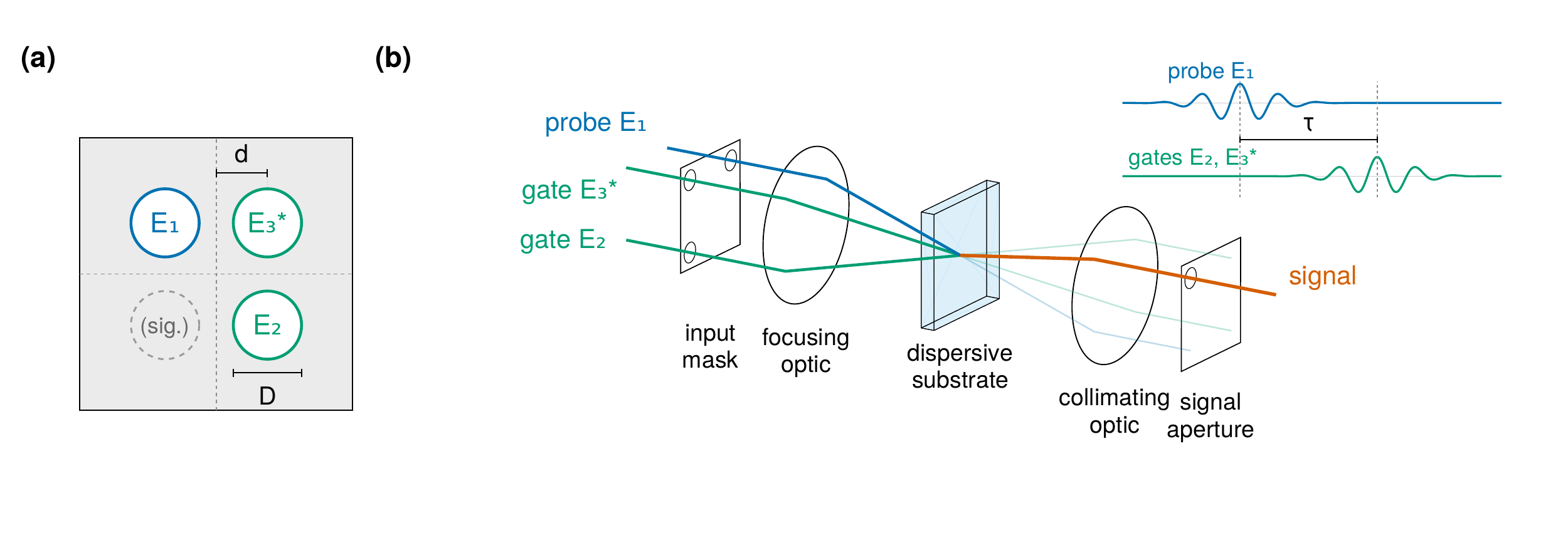
The folded BOXCARS TG-FROG geometry. (a) Mask positions of the probe \(E_1\), the gates \(E_2\) and \(E_3^*\) and the signal, with hole diameter \(D\) and spacing \(d\). (b) The optical chain from the input mask through the dispersive substrate to the signal collection aperture.

Nothing about the measurement is imposed: the transient grating, the phase-matched signal, the geometrical smearing and the chromatic selection by the apertures all emerge from the propagation, independently of the reduced models used for retrieval.

The source pulse, the integrated beamlet spectrum and the on-axis field at the slab entrance are distinct at this bandwidth. All comparisons use the on-axis entrance field as the truth (1.053 fs for the Gaussian series, 1.046 fs for the RDW pulse). The standard and extended models retrieve an effective one-dimensional field, so their complex spectra are converted to the on-axis plane before durations are taken; see field conventions.

The retrieval protocol

All retrievals below use one protocol:

• noise-free simulated scans, with no defringing or baseline subtraction, on a uniform delay core;

• the model re-centred on its own gain-weighted marginal peak at every evaluation, with that centring differentiated — so there is no free delay offset, and neither the smearing scale nor the thickness is fitted;

• lbfgs-ad from a transform-limited start, 400 iterations, objective \(R + 0.03\,P_s + 0.03\,P_a\) (soft spectral constraint and amplitude smoothness);

• for the full model, the collection aperture of the recorded window.

These are not croak’s defaults. The default solver is warm-lbfgs, with reg_spectrum=0.01 and reg_amp=0.03; LM uses a differently normalised objective (see retrieval theory and regularisation). Noise-free simulations need no background treatment; experimental traces need their own preparation.

The failure being fixed

Conventional retrieval fails silently on these measurements. On the simulated RDW pulse at 9.5 µm and a 2 mm collection aperture, the standard thin-medium model fits the trace to \(R = 0.266\,\%\) — a figure normally read as good convergence — and returns 2.433 fs (on-axis; 2.499 fs in its native effective-field convention) for a 1.046 fs pulse: 2.33 times too long. The optimiser absorbs the unmodelled substrate dispersion and geometry into the pulse.

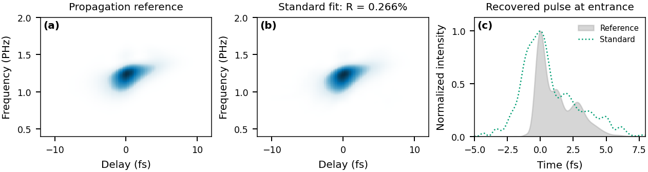
(a) Propagation reference trace for the RDW pulse at 9.5 µm and a 2 mm aperture. (b) The standard-model fit. (c) Its recovered pulse against the reference, both on the on-axis entrance plane. The close fit coexists with a duration overestimate of a factor of 2.33.

The three forward models

Model	Physics	croak options	Use when
standard	single-plane local interaction	defaults	thin medium, multi-cycle pulses
extended	+ dispersive slab + BOXCARS smearing kernel	material=…, smearing=…	multi-cycle pulses, or near-complete collection
full	+ chromatic focal mixture + modelled collection aperture	focal=…, collection=…	octave bandwidth through a restrictive collection aperture

See the forward model, geometric smearing and collection aperture for the equations and configuration. The extended model costs about the same as the standard one; the full model costs minutes rather than seconds per retrieval on a CPU.

Retrieval versus substrate thickness

The central result. Each trace of the Gaussian series — fifteen thicknesses from 1 to 40 µm through a 0.5 mm collection aperture — is retrieved with all three models under the protocol above.

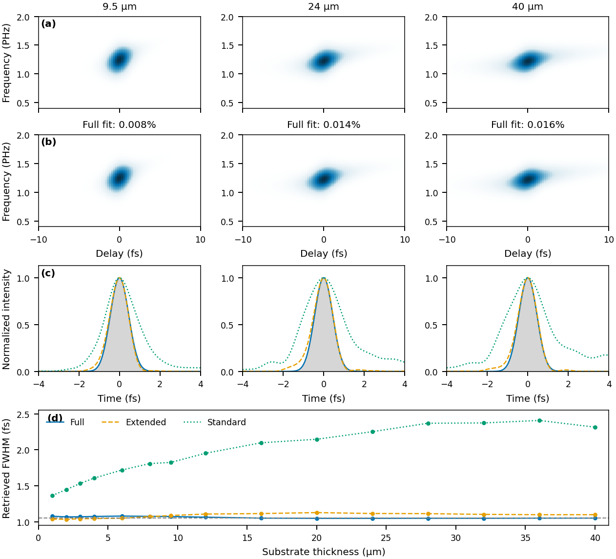
Gaussian thickness series at a 0.5 mm aperture. (a) Reference traces and (b) full-model fits at 9.5, 24 and 40 µm. (c) Temporal profiles of the three models against the reference (grey) on the on-axis entrance plane. (d) Retrieved FWHM at every thickness; the dashed line is the 1.053 fs reference.

The full model retrieves 1.047–1.079 fs against the 1.053 fs reference at every thickness from 1 to 40 µm, at trace residuals of 0.0045–0.0195 %. The standard model returns 1.35–2.41 fs, broadening with thickness (1.36–2.41 fs after conversion to the on-axis plane), while its residual stays below 0.54 %. The extended model removes most of the standard model’s error — its profiles are close to the reference throughout — but at this restrictive aperture a frequency-independent timing kernel still omits the chromatic selection that the full model represents.

Once the measurement physics is in the forward model, substrate thickness stops being the constraint it is in conventional practice: across the tested range a 40 µm substrate retrieves as accurately as a 1 µm one.

Structured pulses and dispersion metrology

A symmetric transform-limited pulse is a limited test of phase retrieval, so the study also retrieves pulses with imposed GDD of ±2 fs² and TOD of +2 fs³.

• The full model recovers both signs of GDD: +1.975 and −1.991 fs² at 9.5 µm, and −2.43 fs² at 40 µm. One case fails: the −2 fs² pulse at 2 µm, where the selected result has −0.98 fs² and a large spurious TOD despite a small residual.

• The TOD case gives 2.04 fs³ for 2 fs³ at 9.5 µm and keeps the trailing satellites. It uses spectral weight 0.01 rather than 0.03.

• The extended model visibly misses the +2 fs² profile at 9.5 µm, and its GDD is biased with thickness (about +1.4 and −3.5 fs² at 40 µm).

• The standard model does not determine the dispersion at this bandwidth: its fitted GDD wanders far from the truth (−7 fs² for −2 fs² at 28 µm).

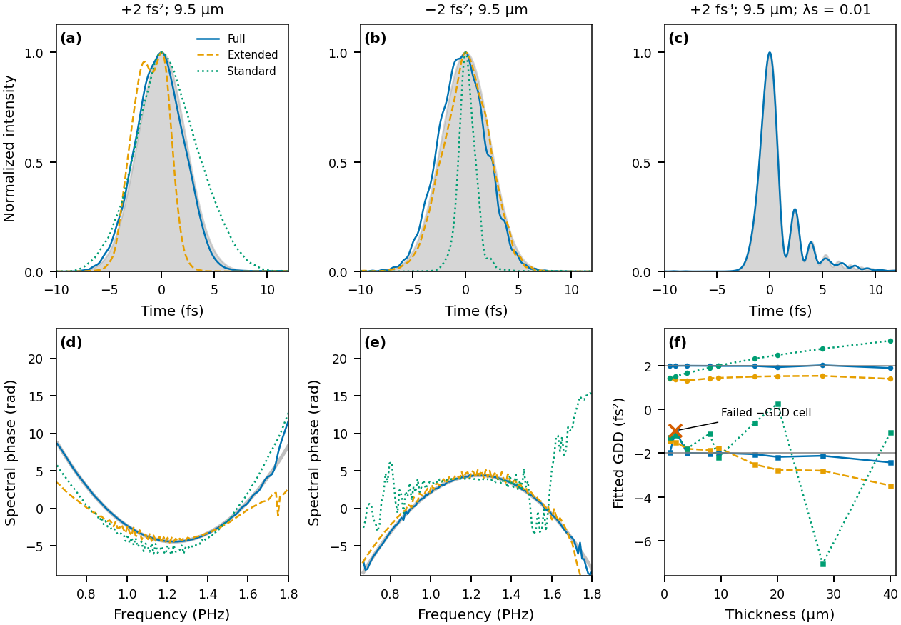
Structured pulses at a 0.5 mm aperture, on the on-axis entrance plane. (a)–(c) Temporal profiles for +2 fs², −2 fs² and +2 fs³ at 9.5 µm against the reference (grey); the extended model visibly fails the +2 fs² profile in (a). (d), (e) Spectral phases of the GDD cases. (f) Fitted GDD versus thickness: the full model tracks ±2 fs² except for the marked −2 fs² failure at 2 µm; the extended model is biased (about +1.4 and −3.5 fs² at 40 µm) and the standard model is far off (−7 fs² at 28 µm). The TOD case uses spectral weight 0.01.

FWHM, polynomial phase coefficients, temporal profiles and complex-field errors answer different questions; report more than one when the truth is known. FWHM can change abruptly when a satellite or shoulder crosses half maximum.

Beam geometry: two timing coordinates

In a focused non-collinear geometry the relative arrival time of the beams varies across the focal spot. In the achromatic, fully collected limit this reduces exactly to two timing coordinates: the gate splitting \(p\) and the probe-to-gate-centroid offset \(\delta\). For an ideal circular-hole BOXCARS mask their widths scale with \((d/D)\,\lambda/c\) — the focal length cancels — and croak.smearing implements the resulting two-parameter kernel. The smearing guide derives and applies these coordinates, including their correlation.

The two coordinates act differently. \(\delta\) translates the trace along delay, so averaging over it is a convolution. Gate splitting is not: for a transform-limited Gaussian it only attenuates the gate, for other transform-limited fields it changes the gate’s shape, and for a chirped Gaussian it shears the trace in frequency. The joint distribution of \((p,\delta)\) is needed to describe both effects.

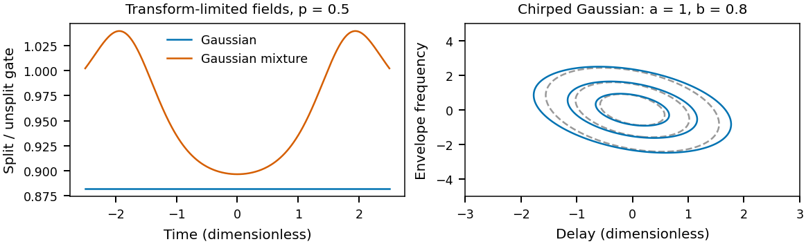
Left: ratio of the split gate \(G(t+p/2)\,G(t-p/2)\) to the unsplit \(G(t)^2\) at splitting \(p=0.5\) (in the same dimensionless time units), for a transform-limited Gaussian \(e^{-t^2}\) and a Gaussian mixture \(e^{-t^2}+0.2\,e^{-t^2/4}\). Only the Gaussian ratio is constant in time. Right: a chirped Gaussian \(E(t)\propto\exp[-(a-ib)t^2/2]\) with \(a=1\), \(b=0.8\) (dimensionless): contours at 0.2, 0.5 and 0.8 of peak of the trace without the timing kernel (dashed grey) and after averaging over a correlated Gaussian \((p,\delta)\) kernel (solid). The kernel broadens the trace along both delay and frequency.

croak’s reduced model shows what ignoring the kernel costs. The geometric smearing example synthesises a 1 fs pulse at 260 nm with the kernel and retrieves it with and without it. With the kernel at its parameter-free geometric value the pulse is recovered exactly. Without it the trace cannot be fitted: the residual grows steadily with the mask ratio \(d/D\), from \(2.4\times10^{-3}\) at \(d/D=0.5\) to \(1.1\times10^{-2}\) at \(d/D=1.25\), and the missing blur is pushed into low-level temporal wings. The FWHM alone is a poor indicator of the error.

The collection aperture: two validated routes

At octave bandwidth the collection aperture is an optical element in its own right: it selects a coherent part of the spatial signal before the squared modulus is integrated, which reshapes the trace along delay in a way a fitted spectral response cannot absorb. The RDW series was recorded through 0.5 and 2 mm apertures at every thickness. Measured as the peak-aligned, peak-normalised rms error of the temporal profile over ±6 fs (not a fractional duration error):

Aperture	Full	Extended	Standard
0.5 mm	0.012–0.045	up to 0.123	up to 0.277
2 mm	0.012–0.046	0.011–0.037	0.239 at 9.5 µm

Two routes therefore work. Hardware: open the collection aperture, and the extended model is adequate — at 2 mm it matches the full model. Software: keep a restrictive aperture and retrieve with the full model. Opening the aperture is bounded by pump leakage into the collection window; the collection guide explains the geometry and the clearance limit.

A simulated single-cycle pulse

The RDW input is the simulated resonant-dispersive-wave emission of a hollow-capillary-fibre source: about 1 fs, with a structured spectrum and trailing satellites. It is injected into the virtual instrument exactly as a measurement would receive it.

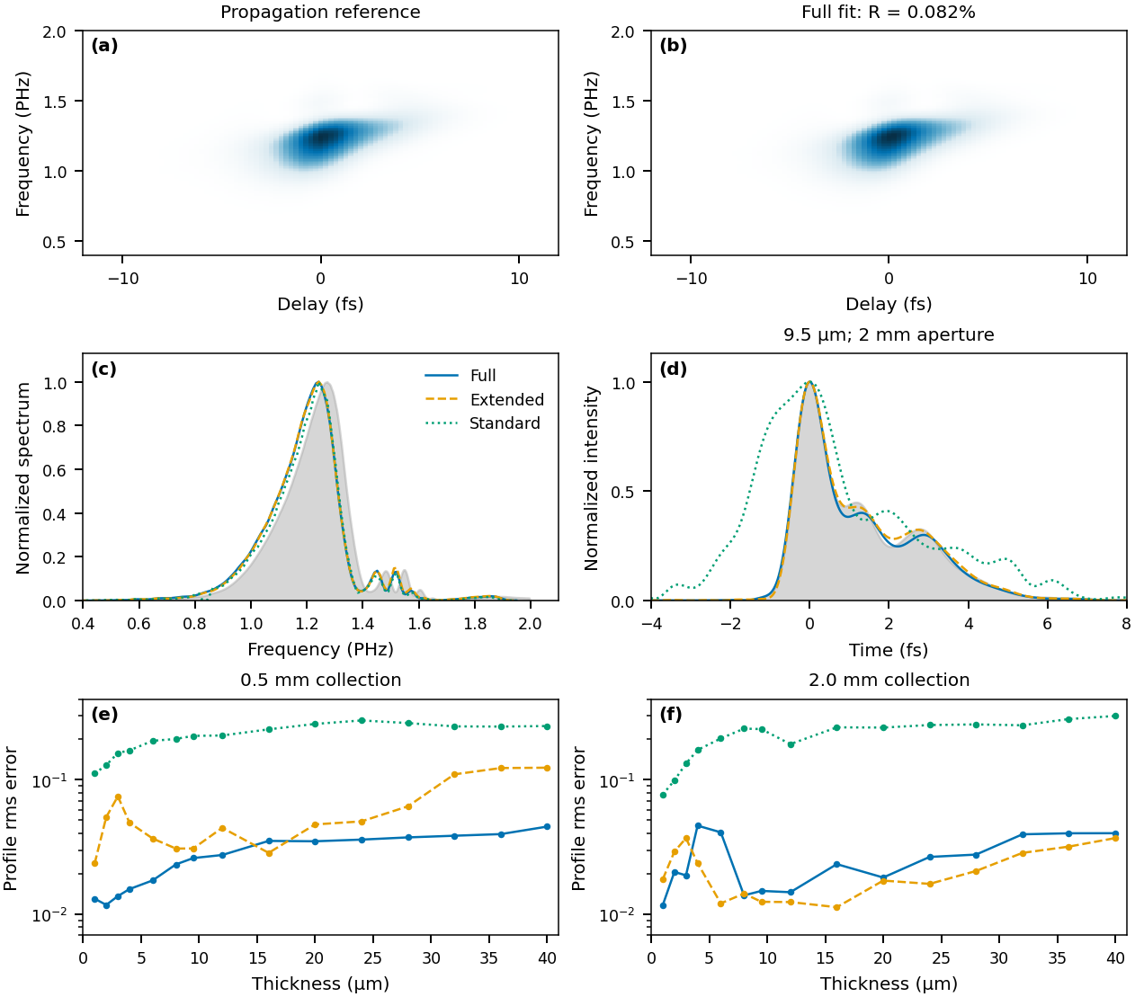
The simulated RDW pulse. (a) Reference trace and (b) full-model fit (\(R=0.082\,\%\)) at 9.5 µm and a 2 mm aperture. (c) Spectra and (d) temporal profiles of the three models against the reference (grey), on the on-axis entrance plane. (e), (f) Profile rms error over ±6 fs versus thickness at 0.5 and 2 mm apertures.

At 9.5 µm and 2 mm, the full model gives 1.054 fs against the 1.046 fs reference, and both the full and extended models reproduce the central peak and its satellites (profile errors 0.0149 and 0.0124); the standard model returns 2.433 fs with a profile error of 0.2387. The extended model is slightly better than the full model here, consistent with its adequacy at an open aperture.

Fixed-field validation and numerical convergence

The forward-model paper holds the input field and geometry fixed — no pulse optimisation — and compares model predictions with sixteen propagation traces: Gaussian and RDW fields, four thicknesses from 4 to 40 µm, and 0.5 and 2 mm apertures. It reports two standards: one global gain, which keeps the spectral yield information, and a fitted gain per frequency row, which allows an unknown detector response. Neither fits the pulse or the delay origin.

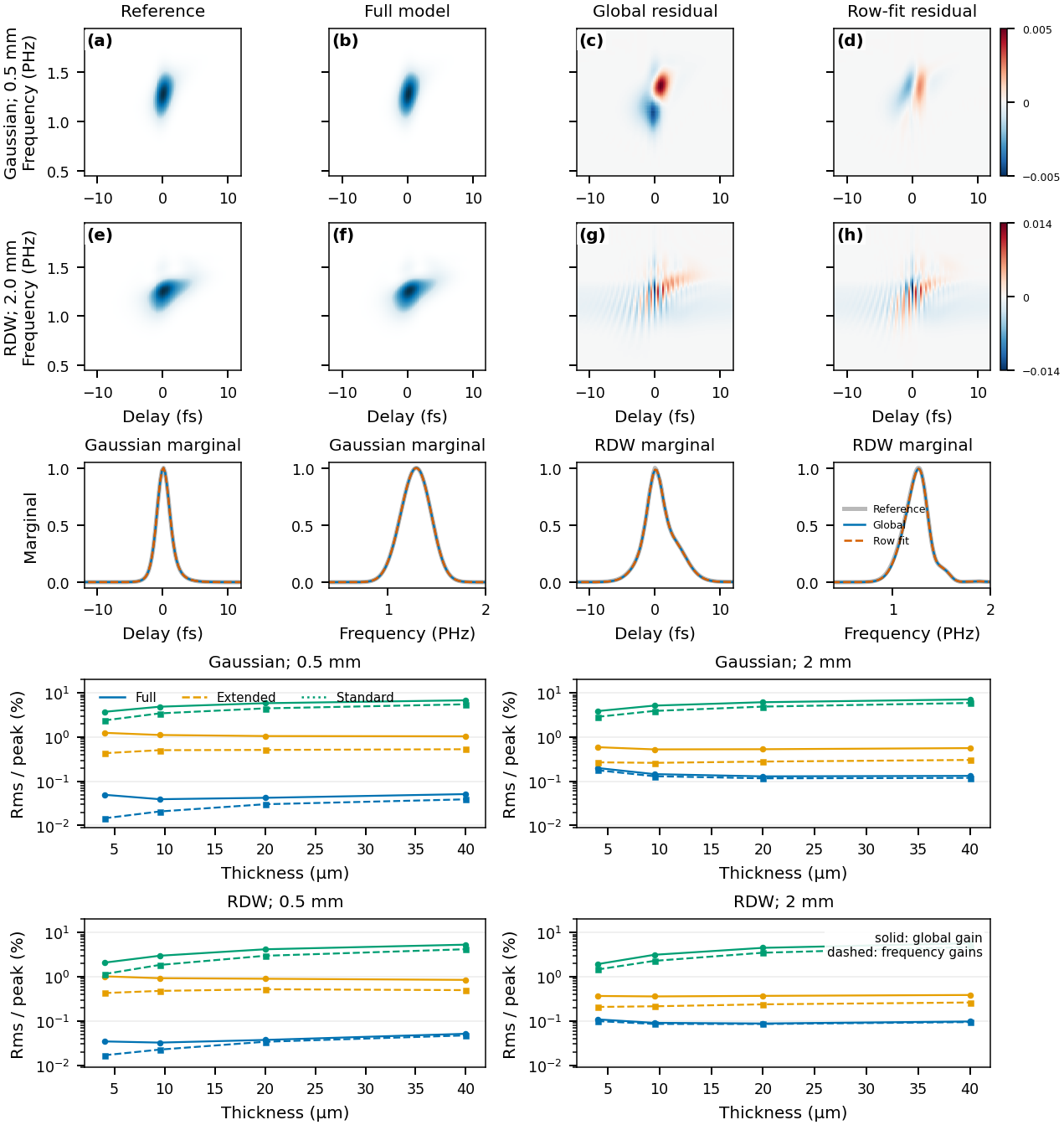
Known-field predictions. (a)–(h) Reference, full-model prediction, and signed residuals with a global gain and with row gains, for the Gaussian at 0.5 mm and the RDW pulse at 2 mm (shared colour scale within each case). Middle row: delay and frequency marginals. Lower panels: rms error per peak versus thickness for the full (blue), extended (orange) and standard (green) model predictions, with a global gain (solid) and row gains (dashed).

The full model reproduces the traces to 0.032–0.200 % rms of peak with a global gain and 0.015–0.178 % with row gains; complete-trace relative-\(L^2\) errors are 0.42–2.48 % (the trace occupies only part of the sampled rectangle, so the two norms differ). The extended and standard predictions, plotted in the lower panels, are clearly worse. The papers’ reference comparison includes the paraxial \(\omega/n\) source-field factor and a declared detector convention; these are properties of that comparison, not of croak’s forward paths. Row gains can absorb a missing spectral factor, so they cannot validate it.

Refining the focal, depth and collection quadrature together changes the full model by at most \(2.8\times10^{-4}\) rms/peak after a global scale; extending the focal radius changes it by about \(1.1\times10^{-6}\).

Solvers and reproducibility

Compare starts, iteration budgets and solvers to separate optimisation error from model error. The −2 fs² failure at 2 µm shows that an accurate forward model does not remove every difficult inverse case, and lowest-residual selection over starts is a protocol choice, not proof of field accuracy. croak’s own solver benchmarks are summarised in algorithms; the algorithm tutorial illustrates solver behaviour and the developer guide describes derivative and implementation checks.

What certifies a retrieval

• The trace error cannot certify the model. The standard model fits every Gaussian trace to below 0.54 % while returning 1.35–2.41 fs for a 1.05 fs pulse. The full-model retrievals reach residuals of 0.0045–0.0195 %, below the 0.032–0.200 % that the same model gives when the true field is pushed through it (the two use different preprocessing, but the point stands): a retrieval can fit the measurement better than the pulse that generated it, by distorting the field to absorb residual model mismatch.

• Validate the forward model with the field held fixed, separately from any retrieval. A smaller retrieval residual is not a substitute.

• Report a retrieval the way it is diagnosed: the measurement model, data support, weights, gains, constraints, reference plane, initialisation and stopping rule alongside the residual; pulse and spectral profiles rather than a single width. If an auxiliary spectrum entered the objective, its agreement is a consistency check, not independent validation. Spread over solver starts measures optimisation sensitivity, not measurement uncertainty — see uncertainty. croak.truth_metrics implements the papers’ error metrics for synthetic and simulated data.

Limits on medium thickness

No upper thickness limit was found: retrieval succeeds over the whole tested range of 1–40 µm; beyond it, numerical resolution, inverse conditioning and focal evolution need assessing again. croak’s models are scalar with an instantaneous nonlinear response.

Reproducing

Two reduced datasets from the simulations ship in examples/data/ (trace, axes and ground truth; see the data README):

uv run python examples/example_paper_thickness.py   # Gaussian series at 4, 9.5 and 40 µm
uv run python examples/example_paper_rdw.py         # the RDW pulse at 9.5 µm

Each retrieves with the extended and standard models and reports trace errors, durations and truth errors, reproducing the qualitative pattern above, including a standard-model fit with a low trace error on a wrong pulse. They use croak’s package defaults with defringing and a fitted delay zero (and, for RDW, a fitted smearing scale), and score the native retrieved fields, so their numbers differ from the papers’. See the gallery and the simulated-trace guide.