Choosing an algorithm

croak has ten solvers behind a single API, grouped into four algorithm families (COPRA, L-BFGS, Levenberg–Marquardt and the global CMA-ES). This tutorial runs three of them on one trace and compares convergence.

import numpy as np
import matplotlib.pyplot as plt
import croak

g = croak.Grid(256, dt=0.5e-15)
ew = croak.gaussian_pulse(g, 3.0e-15, phases=[6e-30, 30e-45])   # GDD + TOD
delays = np.linspace(-24e-15, 24e-15, 90)
trace = croak.maketrace(g.omega, delays, ew, "pg")              # PG-FROG

Run several algorithms

We seed every solver from the same initial guess so the comparison is fair, and record the convergence history res.errors.

Note

The gradient and LM solvers apply croak’s default regularisation weights by default; COPRA takes no penalties. This comparison passes reg_amp=0 so that all three seek minima of the bare trace discrepancy, using either \(R\) or \(R^2\). Those objectives have the same minimisers without penalties but different local geometry.

guess = croak.gaussian_pulse(g, 2.0e-15)     # a deliberately rough start

results = {}
for algo in ("copra", "lbfgs", "lm"):
    kw = {} if algo == "copra" else {"reg_amp": 0}   # COPRA takes no penalties
    results[algo] = croak.retrieve(trace, g.omega, delays, "pg",
                                  algorithm=algo, guess=guess, maxiters=200,
                                  rng=np.random.default_rng(0), progress=False,
                                  **kw)

for algo, res in results.items():
    print(f"{algo:6s}  R = {res.error:.2e}  ({len(res.errors)} evaluations)")

copra   R = 2.64e-06  (200 evaluations)
lbfgs   R = 4.43e-05  (200 evaluations)
lm      R = 1.12e-06  (21 evaluations)

Compare the printed residuals and histories; the next sections explain the differences.

Convergence trajectories

fig, ax = plt.subplots(figsize=(5.5, 4))
for algo, res in results.items():
    ax.semilogy(np.arange(1, len(res.errors) + 1), res.errors, label=algo)
ax.set_xlabel("iteration / evaluation")
ax.set_ylabel("trace error R")
ax.set_title("convergence")
ax.legend()
fig.tight_layout()

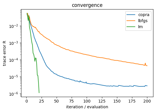
(The x-axis counts iterations for COPRA and objective evaluations for the others, so compare shapes rather than absolute counts.)

Why LM stops early

LM stopped after about 20 evaluations at \(R \approx 10^{-6}\), well short of its 200-evaluation budget, so the budget is not what ended it: a convergence tolerance did. LM uses SciPy’s trust-region reflective method by default, with a JAX Jacobian, and stops as soon as any of its tests passes. croak’s reltol maps to SciPy’s ftol (relative change of the cost), while abstol maps to both xtol (relative step size) and gtol (gradient). Vary them separately to see which one fires:

def lm_run(**tol):
    return croak.retrieve(trace, g.omega, delays, "pg", algorithm="lm",
                          guess=guess, maxiters=400, reg_amp=0, progress=False,
                          **tol)

def describe(r):
    return f"R = {r.error:.2e}  ({len(r.errors)} evaluations)"

print("vary reltol (ftol), abstol at its 1e-8 default:")
for reltol in (1e-4, 1e-8, 1e-12):
    print(f"   reltol={reltol:.0e}  {describe(lm_run(reltol=reltol, abstol=1e-8))}")

print("vary abstol (xtol and gtol), reltol at its 1e-4 default:")
by_abstol = {abstol: lm_run(reltol=1e-4, abstol=abstol)
             for abstol in (1e-8, 1e-12, 1e-15)}
for abstol, r in by_abstol.items():
    print(f"   abstol={abstol:.0e}  {describe(r)}")

vary reltol (ftol), abstol at its 1e-8 default:
   reltol=1e-04  R = 1.12e-06  (21 evaluations)
   reltol=1e-08  R = 1.12e-06  (21 evaluations)
   reltol=1e-12  R = 1.12e-06  (21 evaluations)
vary abstol (xtol and gtol), reltol at its 1e-4 default:
   abstol=1e-08  R = 1.12e-06  (21 evaluations)
   abstol=1e-12  R = 9.85e-10  (30 evaluations)
   abstol=1e-15  R = 3.64e-10  (400 evaluations)

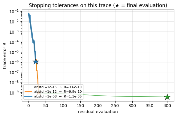
Tightening reltol changes nothing: the cost-change test never fires first. The step/gradient test set by abstol is the one that stops LM here. Tightening it from 1e-8 to 1e-12 lowers \(R\) by about three orders of magnitude, from \(1.1 \times 10^{-6}\) to \(9.9 \times 10^{-10}\), for roughly 1.4× the evaluations. At 1e-15 the test never passes, so LM runs to the 400-evaluation cap for only a further factor of about three. To get more out of LM on a clean trace, tighten abstol, not reltol; around 1e-12 is enough here. The histories of the abstol runs above:

fig, ax = plt.subplots(figsize=(6, 4))
styles = {1e-15: (1.2, "C2"), 1e-12: (2.2, "C1"), 1e-8: (3.5, "C0")}
for abstol, (lw, color) in styles.items():
    r = by_abstol[abstol]
    n = np.arange(1, len(r.errors) + 1)
    ax.semilogy(n, r.errors, lw=lw, color=color, alpha=0.85,
                label=f"abstol={abstol:.0e}  →  R={r.error:.1e}")
    ax.plot(n[-1], r.errors[-1], "*", ms=16, color=color, mec="k", mew=0.5, zorder=5)
ax.set_xlabel("residual evaluation")
ax.set_ylabel("trace error R")
ax.set_title("Stopping tolerances on this trace (★ = final evaluation)")
ax.legend(fontsize=8, loc="lower left")
ax.grid(alpha=0.3)
fig.tight_layout()

Objective shape near an exact fit

Perturb the generating field and compare \(R\) with \(R^2\). This isolates local objective shape from the behaviour of a particular optimiser:

from croak.metrics import trace_error

rng = np.random.default_rng(0)
direction = rng.standard_normal(ew.shape) + 1j * rng.standard_normal(ew.shape)
direction /= np.linalg.norm(direction)
scale = np.linalg.norm(ew)

print(f"{'eps':>8} {'R':>11} {'R/eps':>8} {'R^2/eps^2':>10}")
for eps in (1e-1, 1e-2, 1e-3, 1e-4):
    perturbed = ew + eps * scale * direction
    R = trace_error(trace, croak.maketrace(g.omega, delays, perturbed, "pg"))
    print(f"{eps:8.0e} {R:11.3e} {R / eps:8.4f} {R**2 / eps**2:10.6f}")

     eps           R    R/eps  R^2/eps^2
   1e-01   1.029e-03   0.0103   0.000106
   1e-02   1.005e-04   0.0100   0.000101
   1e-03   1.003e-05   0.0100   0.000101
   1e-04   1.003e-06   0.0100   0.000101

R/eps is constant: the trace error grows linearly with the distance from the solution. On log axes that is a straight line of slope 1, against slope 2 for \(R^2\):

eps = np.logspace(-5, -0.5, 25)
R = np.array([trace_error(trace, croak.maketrace(g.omega, delays,
                                                 ew + e * scale * direction, "pg"))
              for e in eps])

fig, ax = plt.subplots(figsize=(5.5, 4))
ax.loglog(eps, R, "o-", ms=3, label=r"$R$  — what L-BFGS minimises")
ax.loglog(eps, R**2, "s-", ms=3, label=r"$R^2$  — what LM minimises")
ax.loglog(eps, 0.01 * eps, "k--", lw=1, label="slope 1  (a cone)")
ax.loglog(eps, 1.0e-4 * eps**2, "k:", lw=1, label="slope 2  (a paraboloid)")
ax.set_xlabel(r"distance from the solution, $\epsilon$")
ax.set_ylabel("objective")
ax.set_title("the shape of the two objectives at the minimum")
ax.legend(fontsize=8)
fig.tight_layout()

print(f"fitted slopes:  R -> {np.polyfit(np.log(eps), np.log(R), 1)[0]:.3f}"
      f"   R^2 -> {np.polyfit(np.log(eps), np.log(R**2), 1)[0]:.3f}")

fitted slopes:  R -> 1.005   R^2 -> 2.011

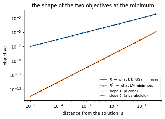
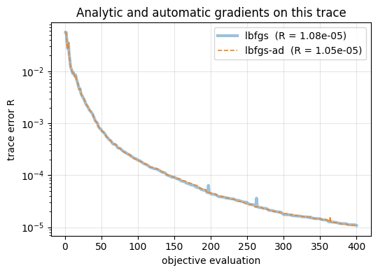
\(R\) is a norm, \(\sqrt{\sum r^2}\), so at a perfect fit it has a \(|x|\)-shaped cusp — a cone, not a paraboloid — and its gradient is undefined at an exact zero. A quasi-Newton line search assumes a smooth local objective, so the cusp limits refinement near an exact fit, whereas the squared residual is smooth. This is why L-BFGS plateaus on a noise-free trace. Compare the analytic and AD routes:

fig, ax = plt.subplots(figsize=(5.5, 4))
for algo, style in (("lbfgs", dict(lw=3.0, alpha=0.45)),
                    ("lbfgs-ad", dict(lw=1.2, ls="--"))):
    r = croak.retrieve(trace, g.omega, delays, "pg", algorithm=algo, guess=guess,
                      maxiters=400, reltol=1e-12, abstol=1e-15, reg_amp=0,
                      progress=False)
    ax.semilogy(np.arange(1, len(r.errors) + 1), r.errors,
                label=f"{algo}  (R = {r.error:.2e})", **style)
ax.set_xlabel("objective evaluation")
ax.set_ylabel("trace error R")
ax.set_title("Analytic and automatic gradients on this trace")
ax.legend()
ax.grid(alpha=0.3)
fig.tight_layout()

Add measurement noise

Noise moves the best achievable residual away from an exact zero. The next calculation adds seeded Gaussian noise and clips negative samples, then compares the same unregularised fits.

noise = np.random.default_rng(1).standard_normal(trace.shape)
noisy = np.clip(trace + 0.01 * trace.max() * noise, 0.0, None)

def centre(t, intensity):
    i = int(np.argmax(intensity))
    return (t - t[i]) * 1e15, intensity / intensity.max()

fig, (ax_conv, ax_pulse) = plt.subplots(1, 2, figsize=(10, 4))
ax_pulse.plot(*centre(g.t, np.abs(g.ifft(ew)) ** 2),
              lw=4, alpha=0.35, color="k", label="true")

for algo in ("copra", "lbfgs", "lm"):
    kw = dict(reltol=1e-12, abstol=1e-15, reg_amp=0) if algo != "copra" else {}
    r = croak.retrieve(noisy, g.omega, delays, "pg", algorithm=algo, guess=guess,
                      maxiters=400, rng=np.random.default_rng(0), progress=False,
                      **kw)
    ax_conv.semilogy(np.arange(1, len(r.errors) + 1), r.errors,
                     label=f"{algo}  (R = {r.error:.3e})")
    ax_pulse.plot(*centre(r.t, r.intensity_t), lw=1.4, label=algo)

ax_conv.set_xlabel("iteration / evaluation")
ax_conv.set_ylabel("trace error R")
ax_conv.set_title("1 % noise: compare residuals")
ax_conv.legend(fontsize=8)
ax_conv.grid(alpha=0.3)
ax_pulse.set_xlim(-15, 15)
ax_pulse.set_xlabel("time (fs)")
ax_pulse.set_ylabel("intensity (norm.)")
ax_pulse.set_title("Compare retrieved pulse profiles")
ax_pulse.legend(fontsize=8)
fig.tight_layout()

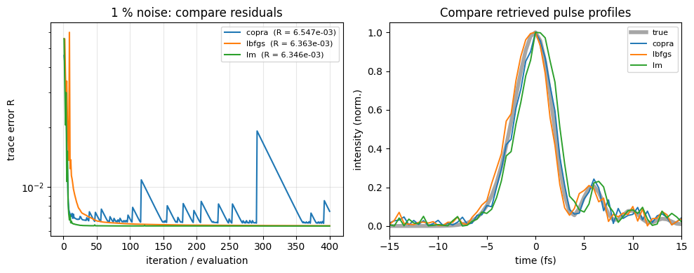
Compare the profiles even if the residuals are similar. Weakly constrained field changes can have little effect on the trace. COPRA’s history can be nonmonotonic because local steps need not reduce the full residual. For a measurement, test starts, physical model and constraints, then assess uncertainty under a justified noise model.

Comparing the two gradient routes

lbfgs-ad takes its gradient from automatic differentiation of the forward model — the general route, and the one that reaches smearing, the fitted extras and the B-spline basis. lbfgs is the same optimiser on the hand-derived adjoint, which covers the core model. The developer validation guide describes direct derivative checks.

hand = croak.retrieve(trace, g.omega, delays, "pg",
                     algorithm="lbfgs", guess=guess, maxiters=120, reg_amp=0,
                     progress=False)
auto = croak.retrieve(trace, g.omega, delays, "pg",
                     algorithm="lbfgs-ad", guess=guess, maxiters=120, reg_amp=0,
                     progress=False)
print(f"lbfgs     R = {hand.error:.3e}")
print(f"lbfgs-ad  R = {auto.error:.3e}")

lbfgs     R = 1.388e-04
lbfgs-ad  R = 1.405e-04

Takeaways

Choose a solver for the required model, constraints and measured convergence. Compare like objectives and record stopping settings. Use warm starts or several starts on non-convex problems. Follow solver selection for model support and interpreting results before reporting a pulse.