Dispersion tuning#
Once you have a retrieved pulse you often want to ask: how short could it be if I
removed its residual chirp? croak.dispersion applies Taylor and material
dispersion to a spectrum and auto-tunes it to maximise the temporal peak power —
as one measure of compression. Peak power, FWHM and satellite energy need not
be optimised by the same phase. Start with the first retrieval
and propagation guide.
import numpy as np
import matplotlib.pyplot as plt
import croak

def center(t, intensity):
    i = int(np.argmax(intensity))
    return t - t[i], intensity / intensity.max()

def temporal_intensity(grid, ew):
    return np.abs(grid.ifft(ew)) ** 2

g = croak.Grid(512, dt=0.5e-15)
omega0 = croak.maths.wlfreq(800e-9)
A chirped pulse#
We generate and retrieve a synthetic pulse with known GDD and TOD. Its time window contains the pulse and scanned delays without wrapping the main signal.
ew_true = croak.gaussian_pulse(g, 5e-15, phases=[40e-30, 300e-45])
delays = np.linspace(-60e-15, 60e-15, 90)
trace = croak.maketrace(g.omega, delays, ew_true, "pg")

res = croak.retrieve(trace, g.omega, delays, "pg", algorithm="copra",
                    maxiters=250, omega0=omega0, rng=np.random.default_rng(0))
I_retr = temporal_intensity(g, res.spectrum)
print(f"trace error R  = {res.error:.2e}")
print(f"retrieved FWHM = {croak.maths.fwhm(*center(g.t, I_retr)) * 1e15:.2f} fs")
retrieval complete — copra / pg
  final error R    : 0.0017%
  retrieved FWHM   : 9.48 fs
  transform limit  : 5.10 fs
  iterations       : 250
  time taken       : 2.87 s
trace error R  = 1.73e-05
retrieved FWHM = 9.48 fs
Auto-compress#
auto_taylor() searches for the (GDD, TOD, FOD) that
maximise the temporal peak power. It never returns a result worse than leaving
the pulse untouched. apply_dispersion() then adds that phase
to the spectrum.
gdd, tod, fod = croak.dispersion.auto_taylor(g, res.spectrum, res.omega0)
print(f"compensating dispersion: GDD = {gdd/1e-30:.0f} fs²,  "
      f"TOD = {tod/1e-45:.0f} fs³")

compressed = croak.apply_dispersion(g.omega, res.omega0, res.spectrum,
                                   gdd=gdd, tod=tod, fod=fod)
I_comp = temporal_intensity(g, compressed)

print(f"peak-power gain  = {I_comp.max() / I_retr.max():.2f}×")
print(f"compressed FWHM  = {croak.maths.fwhm(*center(g.t, I_comp)) * 1e15:.2f} fs")
compensating dispersion: GDD = -40 fs²,  TOD = -298 fs³
peak-power gain  = 2.53×
compressed FWHM  = 5.24 fs
fig, ax = plt.subplots(figsize=(5.5, 4))
for label, I in [("retrieved", I_retr), ("auto-compressed", I_comp)]:
    tc, ic = center(g.t, I)
    ax.plot(tc * 1e15, ic, label=label)
ax.set_xlim(-30, 30)
ax.set_xlabel("time (fs)")
ax.set_ylabel("intensity (norm.)")
ax.set_title("compression by residual-dispersion removal")
ax.legend()
fig.tight_layout()
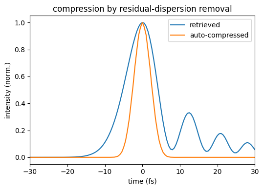
Removing the fitted dispersion flattens the pulse’s spectral phase, concentrating the energy into a shorter, more intense pulse.
From intensity to peak power#
The plots above are normalised, so the “peak-power gain” is a ratio. If you know
the measured pulse energy, pass it to process_result() as
energy= (joules) to read off the absolute peak power in watts. With the
intensity normalised to unit peak, the peak power is energy / ∫I dt — the energy
divided by the effective duration — so compressing the pulse raises it towards the
transform-limited maximum at fixed energy:
pr = croak.process_result(res, measured=trace, energy=100e-6)  # 100 µJ
print(f"peak power     = {pr.peak_power/1e6:.1f} MW")
print(f"TL peak power  = {pr.peak_power_tl/1e6:.1f} MW")  # the maximum achievable
peak power     = 7151.3 MW
TL peak power  = 18450.1 MW
In the GUI’s Dispersion stage this is shown live as you tune the sliders. See Post-processing.
Other knobs#
apply_dispersion() also takes explicit GDD/TOD/FOD if you
want to dial in a known amount, or material_thicknesses / mirror_bounces to
add real glass or mirror dispersion. A negative bounce count removes
(back-propagates) a mirror out of the measured pulse, and beam-path coating mirrors
loaded with load_coating() also divide out their reflectivity.
The corresponding auto-tuner for a material is
auto_material() (e.g. optimal wedge insertion), and you can
register mirrors with register_mirror(). The
Materials and mirrors how-to covers the built-in
chirped mirrors (croak.mirrors.BUILTIN_MIRRORS) and coatings
(croak.mirrors.BUILTIN_COATINGS), building a mirror from your own measurement,
and custom materials.
Sign convention
A positive GDD adds \(+\tfrac12\,\mathrm{GDD}\,\omega^2\) of spectral phase,
matching croak.pulses.gaussian_pulse(). Applying a material’s dispersion and
then its negative cancels exactly.
Next#
Post-processing — the fitted GDD/TOD/FOD report.
croak.dispersionin the API reference.