Your first retrieval#
Retrieve the amplitude and phase of a pulse from a simulated SHG-FROG trace. You will define a pulse, predict its measurement, retrieve it, and interpret the result. A FROG trace is an intensity image indexed by frequency and delay; retrieval infers the complex field that could have produced it.
Start after installation and the Quickstart. The code is executed locally and its outputs are cached with the documentation. These are simulated data with a known answer, not experimental measurements. For the physical background, see measurement fundamentals.
%matplotlib inline
import numpy as np
import matplotlib.pyplot as plt
import croak
A grid and a test pulse#
A croak.grid.Grid carries matched, centred time and angular-frequency axes. We
build a 2.5 fs Gaussian pulse with a little group-delay dispersion (GDD), so its
spectral phase is non-trivial and worth retrieving.
g = croak.Grid(128, dt=0.3e-15)                       # 128 points, 0.3 fs step
omega0 = croak.maths.wlfreq(800e-9)                   # 800 nm carrier
ew = croak.gaussian_pulse(g, 2.5e-15, phases=[4e-30]) # phases = [GDD, TOD, ...] in SI

# the temporal intensity of the true pulse
field_true = g.ifft(ew)
I_true = np.abs(field_true) ** 2
fwhm_true = croak.maths.fwhm(g.t, I_true) * 1e15
print(f"true temporal FWHM = {fwhm_true:.2f} fs")
true temporal FWHM = 5.10 fs
The 2.5e-15 sets the transform-limited width; the 4 fs² of GDD chirps the pulse
and stretches it to the number printed above. Recovering both — the duration and
the chirp that caused it — is the point of the exercise.
For this thin, local model, the carrier omega0 fixes the plotting
wavelength axis \(\lambda = 2\pi c/(\omega+\omega_0)\) used for plotting later.
Synthesise a trace#
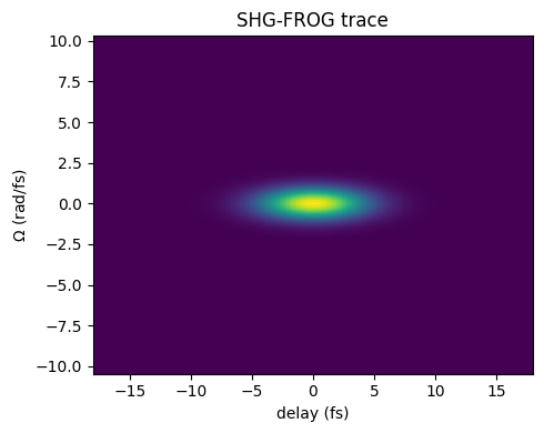
maketrace() runs the forward model
to produce the (Nomega, Ndelay) SHG-FROG trace. The grid is periodic with a
128 × 0.3 fs = 38.4 fs window, and a delay shifts the gate circularly around it.
The ±18 fs scan stays within the ±19.2 fs half-window, so for this few-femtosecond
pulse the shifted gate never wraps round onto the pulse. A longer scan or pulse
needs a longer window (more points or a larger step).
delays = np.linspace(-18e-15, 18e-15, 87)
trace = croak.maketrace(g.omega, delays, ew, "shg")
trace.shape
(128, 87)
fig, ax = plt.subplots(figsize=(5, 4))
ax.imshow(trace, aspect="auto", origin="lower",
          extent=[delays[0] * 1e15, delays[-1] * 1e15,
                  g.omega[0] / 1e15, g.omega[-1] / 1e15])
ax.set_xlabel("delay (fs)")
ax.set_ylabel(r"$\Omega$ (rad/fs)")
ax.set_title("SHG-FROG trace")
fig.tight_layout()
Retrieve#
The retrieve call has a uniform signature
across algorithms. We explicitly choose COPRA,
seeded from a slightly-too-short Gaussian and a fixed random seed so the result is
reproducible. (Passing guess=None instead starts from a random spectrum; on real
data you would run several such random restarts.)
res = croak.retrieve(trace, g.omega, delays, "shg", algorithm="copra",
                    guess=croak.gaussian_pulse(g, 1.8e-15), omega0=omega0,
                    maxiters=300, rng=np.random.default_rng(0), progress=False)
print(f"final trace error R = {res.error:.2e}")
print(f"iterations          = {len(res.errors)}")
final trace error R = 1.08e-16
iterations          = 300
The trace error measures agreement with the supplied intensity trace after fitting its scale. Its interpretation depends on noise, sampling and the forward model; there is no universal threshold that certifies field accuracy. Here we can also compare with the known pulse.
Compare retrieved and true pulse#
Retrieval is defined only up to a trivial time shift and phase, so we peak-centre and peak-normalise both pulses before overlaying them.
def center(t, intensity):
    """Shift so the peak sits at t=0 and normalise the peak to 1."""
    i = int(np.argmax(intensity))
    return t - t[i], intensity / intensity.max()

t_true, I_true_n = center(g.t, I_true)
t_retr, I_retr_n = center(res.t, res.intensity_t)

fig, ax = plt.subplots(figsize=(5, 4))
ax.plot(t_true * 1e15, I_true_n, lw=3, alpha=0.4, label="true")
ax.plot(t_retr * 1e15, I_retr_n, "--", lw=1.5, label="retrieved")
ax.set_xlim(-15, 15)
ax.set_xlabel("time (fs)")
ax.set_ylabel("intensity (norm.)")
ax.legend()
ax.set_title("temporal intensity")
fig.tight_layout()
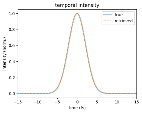
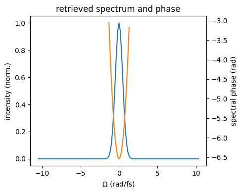
The retrieved intensity overlays the input. The
RetrievalResult also exposes the spectrum, spectral phase
and wavelength axis:
fig, ax = plt.subplots(figsize=(5, 4))
ax.plot(g.omega / 1e15, res.intensity_omega / res.intensity_omega.max(),
        label="spectral intensity")
ax2 = ax.twinx()
mask = res.intensity_omega > 0.02 * res.intensity_omega.max()
ax2.plot(g.omega[mask] / 1e15, res.phase_omega[mask], "C1", label="phase")
ax.set_xlabel(r"$\Omega$ (rad/fs)")
ax.set_ylabel("intensity (norm.)")
ax2.set_ylabel("spectral phase (rad)")
ax.set_title("retrieved spectrum and phase")
fig.tight_layout()
The standard summary figure#
plot_retrieval() collects these comparisons and further
diagnostics in one figure. The GUI presents the same types of panels over three
pages. See post-processing for their definitions.
Because this is SHG, one thing has to be settled first. An SHG trace is
exactly unchanged by \(E(t) \to E^*(-t)\), so a pulse and its mirror image fit it
equally well and the solver returns whichever it happened to find. When a known
temporal intensity is asymmetric, resolve_time_direction() can
choose its matching branch. This Gaussian has a symmetric intensity, so that
comparison cannot establish the sign of GDD; the known spectral phase provides
the additional check here. On experimental data an independent time-direction
measurement is needed. The helper is a no-op for PG and SD.
truth = croak.TruthPulse.from_spectrum(g, ew, omega0)
res, flipped = croak.resolve_time_direction(res, truth)
print(f"time direction flipped to match the truth: {flipped}")
time direction flipped to match the truth: False
f0 = omega0 / (2 * np.pi)                       # SHG signal sits at 2*f0
fig = croak.plot_retrieval(res, measured=trace, truth=truth,
                           lam_min=600e-9, lam_max=1100e-9,
                           flim=(2 * f0 - 0.35e15, 2 * f0 + 0.35e15))
fig      # croak builds Figures without pyplot, so return it to display it
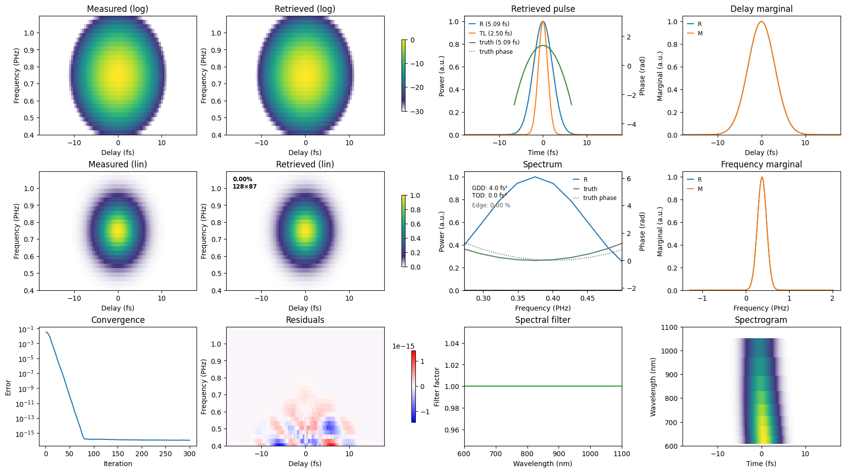
Read it in four groups.
The traces (left block). The supplied and predicted traces appear in linear and logarithmic scales. The log view reveals weak wings that are difficult to see on the linear view. Close agreement shows that the model fits this dataset; it does not by itself establish that the inferred field is correct.
The residual (bottom middle). This is the measured trace minus the scaled prediction, on a symmetric colour scale. Read the colourbar as well as the pattern: a visible structure at numerical round-off is immaterial. At larger amplitudes, structure can indicate calibration, preprocessing, model or convergence problems. The experimental workflow examines an example of a delay-calibration error.
The pulse and spectrum (right block). Compare the retrieved duration with the transform-limited duration for the same spectrum. The fitted GDD has magnitude close to the input 4 fs²; either sign is compatible with this SHG trace. The seeded example shown here reaches the positive-GDD branch, which can be checked against the known spectral phase. Polynomial phase fits depend on the spectral fitting window; inspect the phase itself as well as its coefficients.
Convergence and marginals. The error history shows how the search progressed. Frequency and delay marginals summarise the supplied and predicted traces. Agreement is necessary for a good trace fit but does not establish the phase: different two-dimensional traces can have similar marginals. See marginal checks.
Next#
Compare the solvers on the same trace: Choosing an algorithm.
Retrieve through a dispersive medium: Dispersive retrieval.
Clean and retrieve measured data: Experimental workflow.