The experimental workflow

Measured data usually arrives on the instrument’s wavelength and delay axes. This tutorial follows load → clean → retrieve → post-process → plot → save using a synthetic file in that format. It introduces the same stages as the GUI and the gallery’s workflow example. No experimental data are used here; the known pulse lets us check the effects of preparation and calibration. Start after the first retrieval, and consult preparing and checking data as you adapt this sequence to your instrument.

%matplotlib inline
import tempfile
from pathlib import Path

import h5py
import numpy as np
import matplotlib.pyplot as plt

import croak
from croak.maths import wlfreq

A synthetic measurement file

We first fabricate a PG-FROG file on a wavelength axis (nm) and a delay axis (fs), the way a spectrometer + delay stage would record it.

def make_experiment_file(path):
    # The time window (n*dt = 102 fs) must comfortably exceed the delay range plus
    # the pulse extent, or the gated signal wraps around the periodic FFT window
    # and the "measurement" contains a spurious second copy of the pulse.
    g = croak.Grid(256, dt=0.4e-15)
    omega0 = wlfreq(800e-9)
    ew = croak.gaussian_pulse(g, 6e-15, phases=[25e-30])    # chirped, ~13 fs
    delays = np.linspace(-40e-15, 40e-15, 90)
    trace = croak.maketrace(g.omega, delays, ew, "pg")

    omega_abs = g.omega + omega0
    band = (omega_abs > 0.45 * omega0) & (omega_abs < 2.0 * omega0)
    lam = wlfreq(omega_abs[band])
    order = np.argsort(lam)
    # maketrace returns a *frequency* density I_ω. A spectrometer records a
    # *wavelength* density I_λ = I_ω·|dω/dλ|, and load_and_clean multiplies by
    # λ² to undo exactly that — so convert here, or the Jacobian is applied twice.
    trace_lam = croak.preprocess.omega_to_lambda_density(
        trace[band][order, :], lam[order]
    )
    trace_lam = trace_lam / trace_lam.max()     # detector counts: arbitrary units
    with h5py.File(path, "w") as f:
        f["wavelength"] = lam[order] / 1e-9     # nm
        f["delay"] = delays / 1e-15             # fs
        f["trace"] = trace_lam

    # A real setup also records the fundamental spectrum on its own spectrometer.
    # We simulate that additional channel too. The pipeline uses it for the
    # starting guess and, where enabled, spectral regularisation. It is a
    # wavelength density, hence
    # the |dw/dl| = 2*pi*c/lambda^2 Jacobian.
    lam_spec = lam[order]
    Ilam_spec = np.abs(ew[band][order]) ** 2 * 2 * np.pi * croak.constants.C / lam_spec**2
    Ilam_spec = Ilam_spec / Ilam_spec.max()

    with h5py.File(path, "a") as f:
        f["spectrum_wavelength"] = lam_spec / 1e-9
        f["spectrum_intensity"] = Ilam_spec

    # Pick the band from the wavelength marginal at 1e-4 of its peak — i.e. the
    # -40 dB point, which is where the signal actually ends on a log plot. A
    # few-percent cut looks generous on a linear scale and badly clips the wings.
    marg = trace_lam.sum(axis=1)
    sig = np.where(marg > 1e-4 * marg.max())[0]
    lam_nm = lam[order] / 1e-9
    # The generating pulse, retained for comparison with the retrieved field.
    truth = croak.TruthPulse.from_spectrum(g, ew, omega0)
    return lam_nm[sig[0]] * 1e-9, lam_nm[sig[-1]] * 1e-9, truth

workspace = tempfile.TemporaryDirectory(prefix="croak-workflow-")
h5_path = str(Path(workspace.name) / "measurement.h5")
lam_min, lam_max, truth = make_experiment_file(h5_path)
true_fwhm = truth.fwhm
print(f"signal band: {lam_min*1e9:.0f}-{lam_max*1e9:.0f} nm")
print(f"true FWHM  : {true_fwhm/1e-15:.2f} fs   (kept only to check ourselves)")

signal band: 554-1313 nm
true FWHM  : 13.02 fs   (kept only to check ourselves)

Load

croak.io is a generic dataset picker with unit handling, so we read the arrays and convert them to SI.

fd = croak.io.list_datasets(h5_path)
lam = fd.load("wavelength") * croak.io.unit_to_si("nm")
delays = fd.load("delay") * croak.io.unit_to_si("fs")
trace = fd.load("trace")

# the separately measured fundamental spectrum
lam_spec = fd.load("spectrum_wavelength") * croak.io.unit_to_si("nm")
Ilam_spec = fd.load("spectrum_intensity")
trace.shape, lam_spec.shape

((60, 90), (60,))

This simulated file represents detector counts: counts on a wavelength axis, which is not uniform in frequency, against delay.

fig, (ax_lin, ax_log) = plt.subplots(1, 2, figsize=(10, 4), sharey=True)
for ax, data, title in (
    (ax_lin, trace, "as loaded (linear)"),
    (ax_log, 10 * np.log10(np.maximum(trace / trace.max(), 1e-5)), "same, in dB"),
):
    m = ax.pcolormesh(delays * 1e15, lam * 1e9, data, shading="auto",
                      cmap="viridis", vmin=-50 if "dB" in title else None)
    fig.colorbar(m, ax=ax)
    ax.set_xlabel("delay (fs)")
    ax.set_title(title)
    # the chosen band, on *both* panels — the dB one is where you judge it
    ax.axhline(lam_min * 1e9, color="w", ls="--", lw=1)
    ax.axhline(lam_max * 1e9, color="w", ls="--", lw=1)
ax_lin.set_ylabel("wavelength (nm)")
fig.tight_layout()

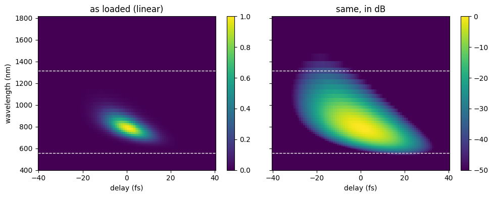
The dashed lines mark the signal band we will keep, and the dB panel is the one to judge them against. On the linear scale the band looks generous; on the log scale you can see how far the trace really extends, and any signal outside the lines is about to be tapered away for good.

Choosing a band from the linear view can discard weak but informative wings. Use the log view together with the measured noise floor; the threshold of \(10^{-4}\) here is a choice for this noise-free simulation, not a universal experimental cutoff. Check td.taper_loss after loading, and repeat a retrieval with a wider band when edge loss is material. A wider band also changes the retrieval grid and computation cost. See grids and filtering for the sampling constraints.

Clean and regrid

load_and_clean() filters and resamples the trace onto a uniform retrieval grid, returning a TraceData. See Preprocessing.

Note what is not in this call. Every filter — the fringe notch, the DC removal, the delay low-pass, the baseline, the noise threshold — is off by default, because each removes real signal along with whatever it targets. Switch one on when your data needs it, not before. The only thing running here is prefilter, the anti-alias low-pass that resampling requires.

td = croak.load_and_clean(
    trace, lam, delays, "pg",
    lam_min=lam_min, lam_max=lam_max, input_unit="delay",
    lam_spec=lam_spec, Ilam_spec=Ilam_spec,      # the independent spectrum
)
print(f"regridded trace: {td.trace.shape[0]} freqs × {td.delays.size} delays")
print(f"retrieval grid : {td.grid.n} points, dt = {td.grid.dt / 1e-15:.2f} fs")

regridded trace: 54 freqs × 90 delays
retrieval grid : 54 points, dt = 3.20 fs

plot_frog_filter() shows the whole cleaning step at once: the measured trace, the filtered version, and what came out on the retrieval grid, in dB on the top row and linear on the bottom.

fig = croak.plot_frog_filter(td)
fig.set_size_inches(11, 5.5)
fig

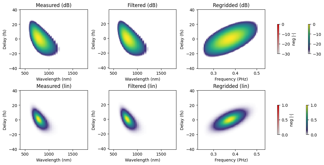
Two things changed. The vertical axis is now angular frequency, uniformly sampled — the retrieval works in \(\omega\), and resampling from \(\lambda\) carries the \(\lambda^2\) Jacobian with it. And the axis has been cropped to the band we asked for, so the empty wavelength ranges above and below the signal no longer occupy rows of the fit. Compare the frequency counts printed above: here the crop removes only 6 of the 60 rows, because this synthetic spectrometer barely samples beyond the signal band. Each forward-model evaluation scales with the number of rows, so the saving is larger on a spectrometer that records a wide empty range around the signal.

Note how little the filtered panel differs from the measured one: with every filter off, the only thing between them is the spectral window. That is what you want on clean data. Each panel also carries a second, white→red colourbar for negative values — croak keeps them rather than clamping to zero, so that a filter which has removed too much is visible instead of silently hidden. Inspect their magnitude relative to the positive signal. Background and filter choices can produce substantial negative values; their presence is a diagnostic, not a reason to clip them silently.

Judge this figure on whether the regridded panel still contains everything the measured one did. Signal clipped at the edges of the band is gone for good — see Grids and filtering for choosing the window.

Retrieve

retrieve_from_tracedata() builds a sensible initial guess from the cleaned trace, picks the solver and runs it.

result = croak.retrieve_from_tracedata(td, algorithm="copra", maxiters=250,
                                      rng=np.random.default_rng(0))
print(f"FROG error R = {result.error:.4%}")

FROG error R = 0.0298%

Always look at the convergence curve before believing a number:

fig, ax = plt.subplots(figsize=(5.5, 3.5))
ax.semilogy(np.arange(1, len(result.errors) + 1), result.errors)
ax.axhline(result.error, color="C1", ls="--", lw=1,
           label=f"best R = {result.error:.2e}")
ax.set_xlabel("iteration")
ax.set_ylabel("trace error R")
ax.set_title("convergence")
ax.legend()
ax.grid(alpha=0.3)
fig.tight_layout()

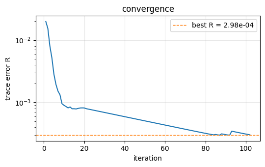
A decreasing curve at the iteration limit suggests further iterations may help. A plateau can reflect convergence, a local minimum, noise, interpolation error or a missing model term. Here regridding changes a trace generated on one grid into samples on another; the interpolated array need not be exactly representable by the retrieval model.

The default retrieval

The call above explicitly chose COPRA. Omitting algorithm uses warm-lbfgs. Since td includes a fundamental spectrum, the default spectral penalty uses it alongside amplitude smoothness (reg_spectrum=0.01, reg_amp=0.03 for this solver). Compare their influence using regularisation; pass both weights as zero for an unregularised fit.

default = croak.retrieve_from_tracedata(td, rng=np.random.default_rng(0))
print(f"warm-lbfgs (default regularisation): R = {default.error:.4%}")

warm-lbfgs (default regularisation): R = 0.0298%

Post-process

process_result() derives display-ready profiles and fits the residual dispersion.

pr = croak.process_result(result, measured=td.trace)
print(f"recovered FWHM = {pr.fwhm_retr / 1e-15:.2f} fs "
      f"(transform-limited {pr.fwhm_tl / 1e-15:.2f} fs)")
print(f"true FWHM      = {true_fwhm / 1e-15:.2f} fs"
      f"   → error {100 * (pr.fwhm_retr - true_fwhm) / true_fwhm:+.1f}%")
print(f"fitted GDD = {pr.gdd_fs2:.0f} fs²,  TOD = {pr.tod_fs3:.0f} fs³"
      f"   (25 fs² went in)")

recovered FWHM = 13.02 fs (transform-limited 6.09 fs)
true FWHM      = 13.02 fs   → error +0.1%
fitted GDD = 25 fs²,  TOD = 0 fs³   (25 fs² went in)

Compare the printed duration and fitted GDD with the known values. Polynomial phase coefficients depend on the phase-fitting band and sampling; inspect the phase curve before interpreting a coefficient. On measured data the generating pulse is unavailable, so result diagnostics and uncertainty analysis become especially important.

Plot

The twelve-panel plot_retrieval() overview shows the measured and retrieved traces, the residual, the temporal and spectral profiles, the marginals and the convergence.

fig = croak.plot_retrieval(result, measured=td.trace, Iomega_meas=td.Iomega,
                          lam_min=td.lam_min, lam_max=td.lam_max,
                          truth=truth, processed=pr)
fig.set_size_inches(11, 8)
fig                                # return the Figure so the notebook displays it

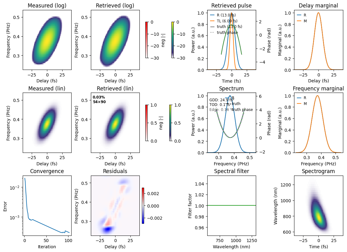
Iomega_meas=td.Iomega overlays the separately recorded fundamental spectrum. In this tutorial it is also used to prepare the initial guess, and the default retrieval above uses it as a spectral constraint. Agreement with that spectrum is therefore a consistency check, not independent validation of the retrieval. truth is available only because this is a simulation. Passing processed=pr reuses the profiles already calculated.

A structured residual can arise from preprocessing as well as missing physics. This trace was generated with the same thin-medium model but interpolated onto a different grid. Before interpreting its residual as evidence for dispersion or spatial effects, test sampling, the selected band, calibration and convergence.

Reading the residual

The residual panel is the most informative thing in that figure, and it repays a systematic look. Structure in it is rarely random: a dipole — a positive lobe beside a negative one — is the signature of a small displacement, because subtracting two copies of the same feature slightly offset from each other leaves exactly that. Correlating the residual against the derivative of the trace along each axis identifies which displacement:

def residual_diagnostics(result, processed, tracedata):
    """Correlate a residual against the shift/scale templates it could arise from."""
    T = result.trace * result.mu
    templates = {
        "delay shift   ∂T/∂τ": np.gradient(T, tracedata.delays, axis=1),
        "freq. shift   ∂T/∂ω": np.gradient(T, tracedata.grid.omega, axis=0),
        "amplitude     T": T,
    }
    a = processed.residual - processed.residual.mean()
    for name, template in templates.items():
        b = template - template.mean()
        c = (a * b).sum() / np.sqrt((a * a).sum() * (b * b).sum())
        print(f"  {name}: {c:+.3f}")

residual_diagnostics(result, pr, td)

  delay shift   ∂T/∂τ: -0.007
  freq. shift   ∂T/∂ω: +0.022
  amplitude     T: +0.066

These correlations test three particular shapes. Small values rule out neither all calibration errors nor missing physics: residual structure orthogonal to these templates remains undetected. Compare them with the deliberate delay shift below.

Time zero is not known a priori on a measured scan; load_and_clean takes it to be where the delay marginal peaks. Reading that off as the largest sample would quantise it to the delay step and leave up to half a step behind, so croak interpolates the peak instead (marginal_peak_delay()). Half a step does not sound like much — here it would be 0.45 fs — but the retrieval sees it clearly. Inject it deliberately and watch:

import dataclasses

step = float(np.diff(td.delays)[0])
shifted = dataclasses.replace(td, delays=td.delays + 0.5 * step)

bad = croak.retrieve_from_tracedata(shifted, algorithm="copra", maxiters=250,
                                    rng=np.random.default_rng(0))
pr_bad = croak.process_result(bad, measured=shifted.trace)
print(f"delay step            = {step / 1e-15:.3f} fs")
print(f"R, correctly centred  = {result.error:.2e}")
print(f"R, offset by half a step = {bad.error:.2e}")
residual_diagnostics(bad, pr_bad, shifted)

delay step            = 0.899 fs
R, correctly centred  = 2.98e-04
R, offset by half a step = 5.10e-03
  delay shift   ∂T/∂τ: -0.534
  freq. shift   ∂T/∂ω: -0.014
  amplitude     T: +0.010

Compare the error and delay-derivative correlation before and after the injected shift. A positive/negative pair of residual lobes is characteristic of a small displacement. Plot both cases on a shared scale:

fig, axes = plt.subplots(1, 2, figsize=(10, 3.6), sharey=True)
vmax = np.abs(pr_bad.residual).max()
for ax, resid, title in (
    (axes[0], pr.residual, f"centred      (R = {result.error:.1e})"),
    (axes[1], pr_bad.residual, f"+half a step (R = {bad.error:.1e})"),
):
    m = ax.pcolormesh(td.delays * 1e15, (td.grid.omega + td.omega0_trace) / (2e15 * np.pi),
                      resid, cmap="bwr", vmin=-vmax, vmax=vmax, shading="auto")
    ax.set_xlabel("delay (fs)")
    ax.set_title(title)
fig.colorbar(m, ax=axes)
axes[0].set_ylabel("frequency (PHz)")

Text(0, 0.5, 'frequency (PHz)')

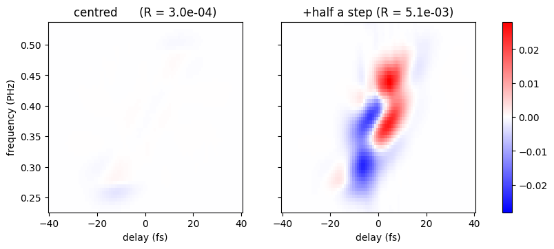
The right panel is the dipole: red on one side of the trace ridge, blue on the other. That antisymmetry across the ridge is what “displaced in delay” looks like, and it is why the correlation test picks out \(\partial T/\partial\tau\).

The autodiff solvers can fit the offset as a free parameter (fit_tau0). This example tests whether fitting an offset accounts for the deliberate displacement:

fixed = croak.retrieve_from_tracedata(shifted, algorithm="lm", fit_tau0=True,
                                      maxiters=400, abstol=1e-14,
                                      rng=np.random.default_rng(0))
print(f"fitted τ₀ = {fixed.tau0 / 1e-15:+.3f} fs   (we injected {0.5 * step / 1e-15:+.3f} fs)")
print(f"R         = {fixed.error:.2e}   (back to the centred value)")

fitted τ₀ = +0.449 fs   (we injected +0.449 fs)
R         = 2.95e-04   (back to the centred value)

Fitting an offset can account for uncertainty in the delay-stage zero, but it adds a parameter that can correlate with the pulse and model geometry. Choose it based on calibration and diagnostic evidence, and inspect the fitted value and its uncertainty. A residual pattern suggests a hypothesis; it does not uniquely identify its cause.

Save

Persist the result (and its processed form) to a portable HDF5 file. See Saving and loading.

out = str(Path(workspace.name) / "retrieval.h5")
croak.save_result(result, out, processed=pr, force=True)
print("wrote", out)

wrote /var/folders/5f/mptc2lq90gb0lnxmd78k9_lh0000gn/T/croak-workflow-a6vgw7mt/retrieval.h5

Choose a permanent output path when analysing your own measurements: this tutorial uses a temporary directory. Save the preparation and retrieval settings as well as the result; sessions support replay and script export.

Continue through the user guide for the assumptions behind each step, or explore data preparation examples for fringe and baseline removal.