Dispersive retrieval#
Propagation inside a nonlinear medium can change a FROG trace substantially. This tutorial predicts a trace for an ultraviolet pulse in fused silica, then compares retrievals with and without the slab’s propagation. It follows your first retrieval.
The recovered pulse is defined at the slab entrance in this one-dimensional model. Generation and retrieval use the same model, so this is a controlled demonstration; the validation chapter tests the models against an independent simulation of the whole instrument, and the model guide explains which to choose.
%matplotlib inline
import numpy as np
import matplotlib.pyplot as plt
import croak
from croak.maths import wlfreq

def center(t, intensity):
    """Peak-centre and peak-normalise (retrieval is defined up to a time shift)."""
    i = int(np.argmax(intensity))
    return t - t[i], intensity / intensity.max()

def fwhm_fs(t, intensity):
    tc, ic = center(t, intensity)
    return croak.maths.fwhm(tc, ic) * 1e15

g = croak.Grid(512, dt=0.3e-15)
omega0 = wlfreq(260e-9)                        # 260 nm carrier
ew = croak.gaussian_pulse(g, 1.5e-15)          # transform-limited, 1.5 fs
delays = np.linspace(-40e-15, 40e-15, 161)

I_true = np.abs(g.ifft(ew)) ** 2
print(f"true temporal FWHM = {fwhm_fs(g.t, I_true):.2f} fs")
true temporal FWHM = 1.51 fs
The input pulse is transform-limited. Any broadening inferred by an inadequate retrieval model in this noise-free example is therefore a retrieval bias. A 1.5 fs pulse at 260 nm is where this matters: its bandwidth is enormous, and fused silica is strongly dispersive in the deep ultraviolet.
A trace through 50 µm of SiO₂#
Passing material, thickness, npoints and the carrier omega0 to
maketrace() models the propagation of both the input and the signal
fields inside the slab. We use the PG interaction (the transient-grating
kernel); dispersive propagation is supported for PG and SD, not SHG.
We use a 50 µm slab. Its small physical thickness does not imply negligible spectral phase across this pulse’s bandwidth:
disp = dict(material="SiO2", thickness=50e-6, npoints=20, omega0=omega0)
print(f"GDD of the slab at 260 nm = "
      f"{croak.dispersion.material_gdd('SiO2', omega0, disp['thickness']):.1f} fs²")

trace = croak.maketrace(g.omega, delays, ew, "pg", **disp)
trace.shape
GDD of the slab at 260 nm = 10.4 fs²
(512, 161)
The time window is 153.6 fs, wide enough to contain the propagated replicas without wrapping them across the periodic boundary. The scan extends to ±40 fs; check its edge signal when adapting the pulse or slab. A successful same-model retrieval cannot diagnose a window that is too short in both generation and fitting.
The printed GDD is the quadratic spectral-phase coefficient at the carrier. The forward model uses the full material dispersion across the sampled band, not only this coefficient.
Check the depth integral while holding the pulse fixed. Doubling its quadrature is a numerical convergence check, separate from retrieval or physical validation:
trace_finer = croak.maketrace(g.omega, delays, ew, "pg", **(disp | {"npoints": 40}))
relative_difference = np.linalg.norm(trace - trace_finer) / np.linalg.norm(trace_finer)
print(f"20 vs 40 depth nodes: relative trace L2 difference = {relative_difference:.2e}")
print(f"delay-edge signal / peak = {trace[:, [0, -1]].max() / trace.max():.2e}")
20 vs 40 depth nodes: relative trace L2 difference = 1.34e-05
delay-edge signal / peak = 4.70e-05
Dispersion-aware retrieval#
The retrieval must use the same dispersive model — pass the slab parameters to
retrieve() as well. We use COPRA here.
near = croak.gaussian_pulse(g, 2.0e-15)
res = croak.retrieve(trace, g.omega, delays, "pg", algorithm="copra",
                    guess=near, maxiters=300, rng=np.random.default_rng(0), **disp)
print(f"trace error R  = {res.error:.2e}")
print(f"recovered FWHM = {fwhm_fs(res.t, res.intensity_t):.2f} fs"
      f"   (true {fwhm_fs(g.t, I_true):.2f} fs)")
retrieval complete — copra / pg
  final error R    : 0.0000%
  retrieved FWHM   : 1.50 fs
  transform limit  : 1.50 fs
  iterations       : 300
  time taken       : 28.00 s
trace error R  = 6.06e-08
recovered FWHM = 1.51 fs   (true 1.51 fs)
The dispersion-aware retrieval recovers the true duration. The full summary shows what that means panel by panel, with the known pulse overlaid:
truth = croak.TruthPulse.from_spectrum(g, ew, omega0)
f0 = omega0 / (2 * np.pi)          # PG is degenerate: signal at the fundamental

fig = croak.plot_retrieval(res, measured=trace, truth=truth,
                           lam_min=200e-9, lam_max=380e-9,
                           flim=(f0 - 0.55e15, f0 + 0.55e15))
fig.set_size_inches(11, 8)
fig                                # return the Figure so the notebook displays it
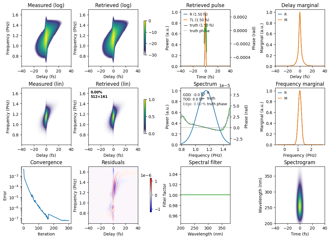
Compare the asymmetric trace with the recovered pulse. Propagation changes the input replicas and the generated signal throughout the slab. The inverse model can attribute that distortion to the known material instead of assigning it to the entrance pulse. Check the duration, spectral phase and residual together. A small residual is expected for this matched, noise-free model; the comparison with the known field is the additional evidence for accuracy in this example.
What a thin-medium model does#
Retrieving the same trace without the slab model — as classic FROG would — misattributes the medium’s dispersion to the pulse.
res_thin = croak.retrieve(trace, g.omega, delays, "pg", algorithm="copra",
                         guess=near, maxiters=300, rng=np.random.default_rng(0))
print(f"thin-model trace error R = {res_thin.error:.2e}")
print(f"thin-model FWHM          = {fwhm_fs(res_thin.t, res_thin.intensity_t):.2f} fs"
      f"   (true {fwhm_fs(g.t, I_true):.2f} fs)")
retrieval complete — copra / pg
  final error R    : 0.3113%
  retrieved FWHM   : 2.78 fs
  transform limit  : 0.67 fs
  iterations       : 300
  time taken       : 7.33 s
thin-model trace error R = 3.11e-03
thin-model FWHM          = 2.77 fs   (true 1.51 fs)
t_true, I_true_n = center(g.t, I_true)
t_disp, I_disp_n = center(res.t, res.intensity_t)
t_thin, I_thin_n = center(res_thin.t, res_thin.intensity_t)

fig, ax = plt.subplots(figsize=(5.5, 4))
ax.plot(t_true * 1e15, I_true_n, lw=3, alpha=0.4, label="true")
ax.plot(t_disp * 1e15, I_disp_n, "--", lw=1.5, label="dispersive model")
ax.plot(t_thin * 1e15, I_thin_n, ":", lw=1.5, label="thin model")
ax.set_xlim(-8, 8)
ax.set_xlabel("time (fs)")
ax.set_ylabel("intensity (norm.)")
ax.legend()
ax.set_title("dispersive vs thin-medium retrieval")
fig.tight_layout()
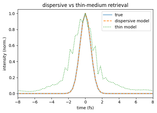
The thin model returns a pulse almost twice as long as the truth — about 2.8 fs for the 1.5 fs pulse. The slab’s dispersion has been misattributed to the pulse, because a thin-medium model has nowhere else to put it. Yet its trace error is around \(3\times10^{-3}\) — 0.3 %, the kind of number usually reported as a well-converged FROG retrieval:
print(f"dispersive model:  R = {res.error:.1e}   FWHM = {fwhm_fs(res.t, res.intensity_t):.2f} fs")
print(f"thin model:        R = {res_thin.error:.1e}   FWHM = {fwhm_fs(res_thin.t, res_thin.intensity_t):.2f} fs")
print(f"truth:                              FWHM = {fwhm_fs(g.t, I_true):.2f} fs")
dispersive model:  R = 6.1e-08   FWHM = 1.51 fs
thin model:        R = 3.1e-03   FWHM = 2.77 fs
truth:                              FWHM = 1.51 fs
A small trace error only means the model reproduces the measurement. It says nothing about whether the model is the right one, and no amount of iterating, no better optimiser and no random restart will supply a missing term in the physics. The defence is to model the medium, which costs one extra keyword.
The effect grows with shorter pulses and deeper into the ultraviolet. In simulations of a complete TG-FROG instrument (validation), a thin-medium model retrieves a 1.05 fs pulse at 260 nm as 1.35–2.41 fs depending on the substrate thickness, at trace errors below 0.54 %, while croak’s full model — the dispersive slab plus the beam geometry and collection aperture — recovers 1.047–1.079 fs at every thickness from 1 to 40 µm. For a real experiment, the beam geometry and collection matter as well as the slab.
Note
The slab parameters are available across the retrieval solvers for PG and SD. Selected solvers can fit thickness and delay zero. Such a fit correlates with the pulse phase, so an independent thickness calibration is better where available. The uncertainty guide explains how uncertainty in the slab propagates to duration.
Next#
Continue with the experimental workflow, or use the instrument examples to explore more detailed models.
The physics: The forward model and validation.
Compress residual dispersion: Dispersion tuning.